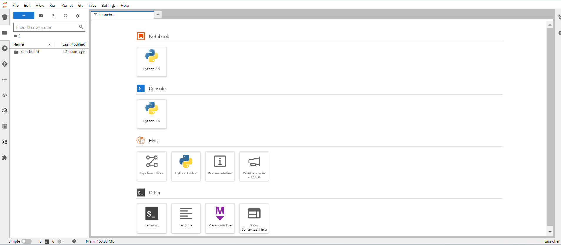
Configure a Jupyter notebook to use GPUs for AI/ML modeling
Prerequisites:
Prepare your Jupyter notebook server for using a GPU, you need to have:
-
Before proceeding, confirm that you have an active GPU quota that has been approved for your current NERC OpenShift Allocation through NERC ColdFront. Read more about How to Access GPU Resources on NERC OpenShift Allocation.
-
Select the correct data science project and create workbench, see Populate the data science project for more information.
Please ensure that you start your Jupyter notebook server with options as depicted in the following configuration screen. This screen provides you with the opportunity to select a notebook image and configure its options, including the Accelerator and Number of accelerators (GPUs).
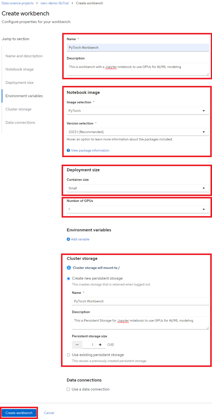
For our example project, let's name it "PyTorch Workbench". We'll select the Jupyter | PyTorch | CUDA | Python 3.12 image, choose a Deployment size of Small, choose Accelerator of NVIDIA V100 GPU, Number of accelerators as 1, and allocate a Cluster storage space of 20GB (Selected By Default).
Hardware Acceleration using GPU
A GPU is highly recommended for this type of training to significantly improve performance and reduce training time.
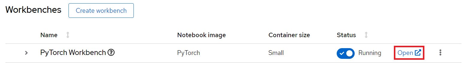
If this procedure is successful, you have started your Jupyter notebook server. When your workbench is ready and the status changes to Running, click the open icon ( ) next to your workbench's name, or click the workbench name directly to access your environment:
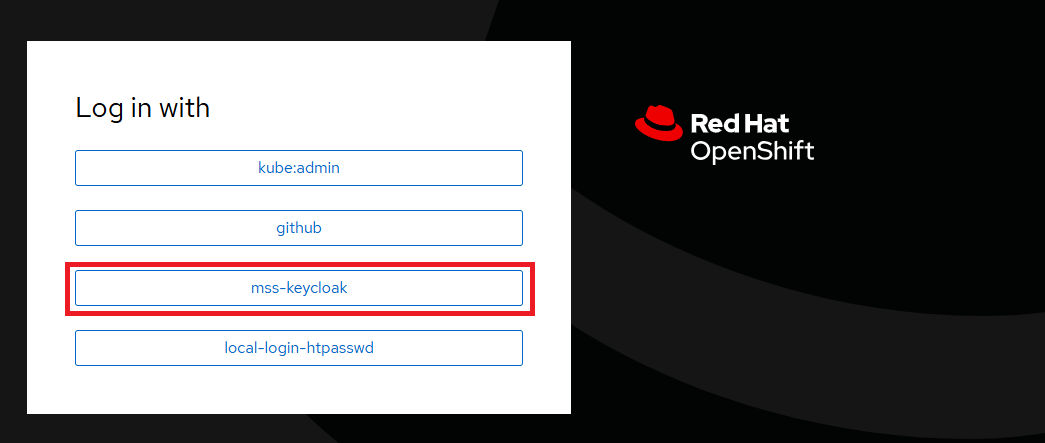
Once you have successfully authenticated by clicking "mss-keycloak" when prompted, as shown below:
Next, you should see the NERC RHOAI JupyterLab Web Interface, as shown below:
The Jupyter environment is currently empty. To begin, populate it with content using Git. On the left side of the navigation pane, locate the Name explorer panel, where you can create and manage your project directories.
Learn More About Working with Notebooks
For detailed guidance on using notebooks on NERC RHOAI JupyterLab, please refer to this documentation.
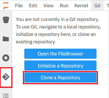
Clone a GitHub Repository
You can clone a Git repository in JupyterLab through the left-hand toolbar or the Git menu option in the main menu as shown below:
Let's clone a repository using the left-hand toolbar. Click on the Git icon, shown in below:

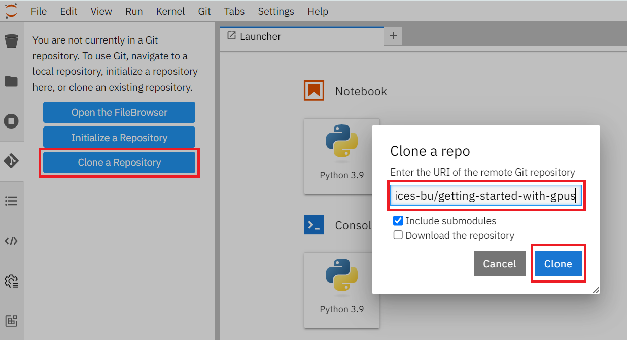
Then click on Clone a Repository as shown below:
Enter the git repository URL, which points to the end-to-end ML workflows demo project i.e. https://github.com/rh-aiservices-bu/getting-started-with-gpus.
https://github.com/rh-aiservices-bu/getting-started-with-gpus
Then click Clone button, as shown below:
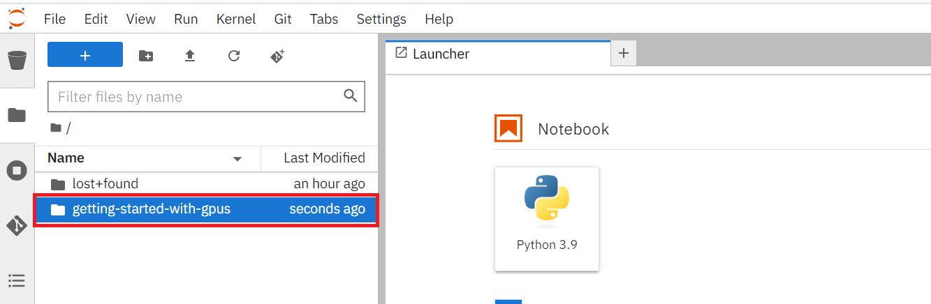
Cloning takes a few seconds, after which you can double-click and navigate to the newly-created folder i.e. getting-started-with-gpus that contains your cloned Git repository.
You will be able to find the newly-created folder named getting-started-with-gpus based on the Git repository name, as shown below:
Exploring the getting-started-with-gpus repository contents
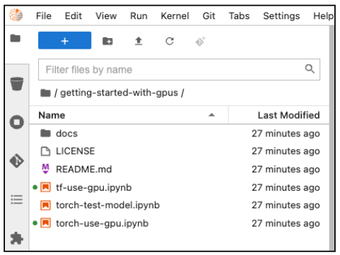
After you've cloned your repository, the getting-started-with-gpus repository contents appear in a directory under the Name pane. The directory contains several notebooks as .ipnyb files, along with a standard license and README file as shown below:
Double-click the torch-use-gpu.ipynb file to open this notebook.
This notebook handles the following tasks:
-
Importing torch libraries (utilities).
-
Listing available GPUs.
-
Checking that GPUs are enabled.
-
Assigning a GPU device and retrieve the GPU name.
-
Loading vectors, matrices, and data onto a GPU.
-
Loading a neural network model onto a GPU.
-
Training the neural network model.
Start by importing the various torch and torchvision utilities:
import torch
import torch.nn as nn
import torch.nn.functional as F
from torch.utils.data import TensorDataset
import torch.optim as optim
import torchvision
from torchvision import datasets
import torchvision.transforms as transforms
import matplotlib.pyplot as plt
from tqdm import tqdm
Once the utilities are loaded, determine how many GPUs are available:
When you have confirmed that a GPU device is available for use, assign a GPU device and retrieve the GPU name:
device = torch.device("cuda:0" if torch.cuda.is_available() else "cpu")
print(device)  # Check which device we got
Once you have assigned the first GPU device to your device variable, you are ready to work with the GPU. Let's start working with the GPU by loading vectors, matrices, and data:
X_train = torch.IntTensor([0, 30, 50, 75, 70])  # Initialize a Tensor of Integers with no device specified
print(X_train.is_cuda, ",", X_train.device)  # Check which device Tensor is created on
# Move the Tensor to the device we want to use
X_train = X_train.cuda()
# Alternative method: specify the device using the variable
# X_train = X_train.to(device)
# Confirm that the Tensor is on the GPU now
print(X_train.is_cuda, ",", X_train.device)
# Alternative method: Initialize the Tensor directly on a specific device.
X_test = torch.cuda.IntTensor([30, 40, 50], device=device)
print(X_test.is_cuda, ",", X_test.device)
After you have loaded vectors, matrices, and data onto a GPU, load a neural network model:
# Here is a basic fully connected neural network built in Torch.
# If we want to load it / train it on our GPU, we must first put it on the GPU
# Otherwise it will remain on CPU by default.

batch_size = 100

class SimpleNet(nn.Module):
    def __init__(self):
        super(SimpleNet, self).__init__()
        self.fc1 = nn.Linear(784, 784)
        self.fc2 = nn.Linear(784, 10)

    def forward(self, x):
        x = x.view(batch_size, -1)
        x = self.fc1(x)
        x = F.relu(x)
        x = self.fc2(x)
        output = F.softmax(x, dim=1)
        return output
After the model has been loaded onto the GPU, train it on a data set. For this example, we will use the FashionMNIST data set:
"""
    Data loading, train and test set via the PyTorch dataloader.
"""
# Transform our data into Tensors to normalize the data
train_transform=transforms.Compose([
        transforms.ToTensor(),
        transforms.Normalize((0.1307,), (0.3081,))
        ])

test_transform=transforms.Compose([
        transforms.ToTensor(),
        transforms.Normalize((0.1307,), (0.3081,)),
        ])

# Set up a training data set
trainset = datasets.FashionMNIST('./data', train=True, download=True,
                  transform=train_transform)
train_loader = torch.utils.data.DataLoader(trainset, batch_size=batch_size,
                                          shuffle=False, num_workers=2)

# Set up a test data set
testset = datasets.FashionMNIST('./data', train=False,
                  transform=test_transform)
test_loader = torch.utils.data.DataLoader(testset, batch_size=batch_size,
                                        shuffle=False, num_workers=2)
Once the FashionMNIST data set has been downloaded, you can take a look at the dictionary and sample its content.
# A dictionary to map our class numbers to their items.
labels_map = {
    0: "T-Shirt",
    1: "Trouser",
    2: "Pullover",
    3: "Dress",
    4: "Coat",
    5: "Sandal",
    6: "Shirt",
    7: "Sneaker",
    8: "Bag",
    9: "Ankle Boot",
}

# Plotting 9 random different items from the training data set, trainset.
figure = plt.figure(figsize=(8, 8))
for i in range(1, 3 * 3 + 1):
    sample_idx = torch.randint(len(trainset), size=(1,)).item()
    img, label = trainset[sample_idx]
    figure.add_subplot(3, 3, i)
    plt.title(labels_map[label])
    plt.axis("off")
    plt.imshow(img.view(28,28), cmap="gray")
plt.show()
The following figure shows a few of the data set's pictures:
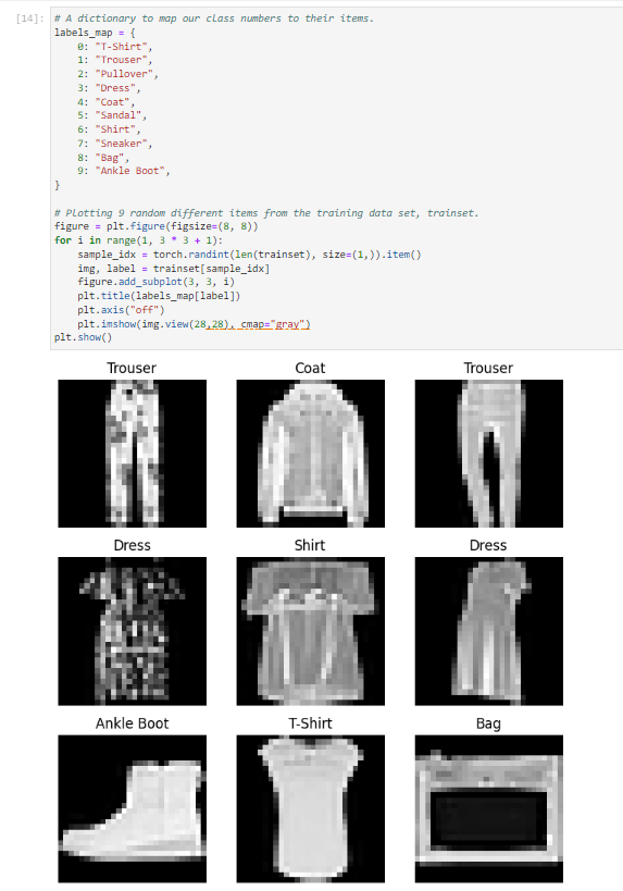
There are ten classes of fashion items (e.g. shirt, shoes, and so on). Our goal is to identify which class each picture falls into. Now you can train the model and determine how well it classifies the items:
def train(model, device, train_loader, optimizer, epoch):
    """Model training function"""
    model.train()
    print(device)
    for batch_idx, (data, target) in tqdm(enumerate(train_loader)):
        data, target = data.to(device), target.to(device)
        optimizer.zero_grad()
        output = model(data)
        loss = F.nll_loss(output, target)
        loss.backward()
        optimizer.step()
def test(model, device, test_loader):
    """Model evaluating function"""
    model.eval()
    test_loss = 0
    correct = 0
    # Use the no_grad method to increase computation speed
    # since computing the gradient is not necessary in this step.
    with torch.no_grad():
        for data, target in test_loader:
            data, target = data.to(device), target.to(device)
            output = model(data)
            test_loss += F.nll_loss(output, target, reduction='sum').item()  # sum up batch loss
            pred = output.argmax(dim=1, keepdim=True)  # get the index of the max log-probability
            correct += pred.eq(target.view_as(pred)).sum().item()

    test_loss /= len(test_loader.dataset)

    print('\nTest set: Average loss: {:.4f}, Accuracy: {}/{} ({:.0f}%)\n'.format(
        test_loss, correct, len(test_loader.dataset),
        100. * correct / len(test_loader.dataset)))
# number of  training 'epochs'
EPOCHS = 5
# our optimization strategy used in training.
optimizer = optim.Adadelta(model.parameters(), lr=0.01)
for epoch in range(1, EPOCHS + 1):
        print( f"EPOCH: {epoch}")
        train(model, device, train_loader, optimizer, epoch)
        test(model, device, test_loader)
As the model is trained, you can follow along as its accuracy increases from 63 to 72 percent. (Your accuracies might differ, because accuracy can depend on the random initialization of weights.)
Once the model is trained, save it locally:
Load and Test the PyTorch model
Let's now determine how our simple torch model performs using GPU resources.
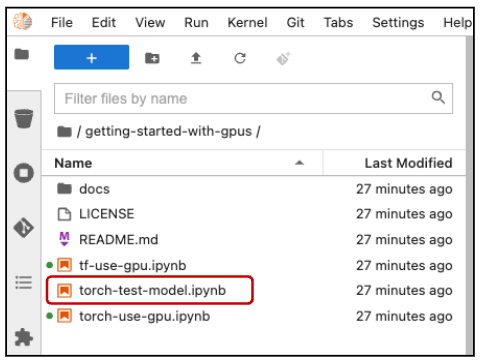
In the getting-started-with-gpus directory, double click on the torch-test-model.ipynb file (highlighted as shown below) to open the notebook.
After importing the torch and torchvision utilities, assign the first GPU to your device variable. Prepare to import your trained model, then place the model on your GPU and load in its trained weights:
import torch
import torch.nn as nn
import torch.nn.functional as F
from torchvision import datasets
import torchvision.transforms as transforms
import matplotlib.pyplot as plt
device = torch.device("cuda:0" if torch.cuda.is_available() else "cpu")
print(device)  # let's see what device we got
# Getting set to import our trained model.

# batch size of 1 so we can look at one image at time.
batch_size = 1


class SimpleNet(nn.Module):
    def __init__(self):
        super(SimpleNet, self).__init__()
        self.fc1 = nn.Linear(784, 784)
        self.fc2 = nn.Linear(784, 10)

    def forward(self, x):
        x = x.view(batch_size, -1)
        x = self.fc1(x)
        x = F.relu(x)
        x = self.fc2(x)
        output = F.softmax(x, dim=1)
        return output
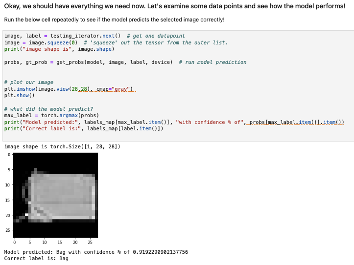
You are now ready to examine some data and determine how your model performs. The sample run as shown below shows that the model predicted a "bag" with a confidence of about 0.9192. Despite the % in the output, 0.9192 is very good because a perfect confidence would be 1.0.